---
title: "Building a simple emulator"
output: html_document
---
```{r setup, include=FALSE}
suppressPackageStartupMessages(library(tidyverse))
knitr::opts_chunk$set(fig.path='Demonstrations/', fig.height=4)
```
#### The simulator
We define a simple function to emulate:
```{r}
simulator = function(x) {
sin(2*x) * exp(-0.5 * x^2)
}
df_simulator = data.frame(x = seq(-3, 3, 0.01), y = simulator(seq(-3, 3, 0.01)))
ggplot(df_simulator, aes(x = x, y = y)) + geom_line()
```
#### The design points
The preliminary step is that we need to identify the possible range of input $x$.
Let's assume that possible range for $x$ is $[-3, 3]$. We need to normalize our input $x$, i.e. from $[-3, 3]$ to $[-1, 1]$. We decided to choose 15 design points and evaluate our simulator at these design points in order to construct GP emulator.
We added the *Noise* term to avoid overfitting our mean function component.
```{r}
tData = data.frame(x = seq(-3, 3, length.out = 15), Noise = rnorm(15, 0, 0.4),
y = simulator(seq(-3, 3, length.out = 15)))
# Normalize your input x to [-1, 1]
tData$x = 2*(tData$x - min(tData$x))/(max(tData$x) - min(tData$x)) - 1
head(tData)
ggplot(tData, aes(x = x, y=y)) + geom_point()
```
#### Building the emulator
Firstly, start with fitting the emulator mean functions. Function **EMULATE.lm** uses the stepwise regression procedure. The functions we consider adding to $g(x)$ are linear, quadratic, cubic and Fouriers transformations with up to third intercations between all parameters. For this simple example we do not need such complicated terms.
```{r eval=FALSE}
cands <- names(tData)[1]
myem.lm <- EMULATE.lm(Response=names(tData)[3], tData=tData,
tcands=cands,tcanfacs=NULL,TryFouriers=FALSE,
maxOrder=2, maxdf = 2)
```
Secondly, you construct the GP emulator with function **EMULATE.gpstan**. We are required to specify *nugget* term, which for this particular example is set to 0.0001 for numerical stability of covariance matrix. Another important function argument is *FastVersion*. In case when the Fully Bayesian analysis is too lengthy, we could fix parameters at their posterior mode values.
```{r eval=FALSE}
myem.gp <- EMULATE.gpstan(meanResponse=myem.lm, nugget=0.0001, tData=tData,
additionalVariables=cands,CreatePredictObject = FALSE,
FastVersion=TRUE)
```
These are two main steps in constructing GP emulator.
#### Validation of GP emulator performance
To validate our GP emulator we produce Leave One Out plots against inputs.
```{r eval =FALSE}
tLOOs <- stanLOOplot(StanEmulator = myem.gp, ParamNames=names(tData)[1])
```
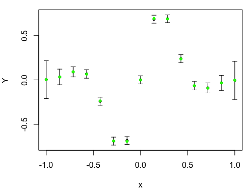 Traditional Leave One Out plot against input $x$. The predictions and two standard deviation prediction intervals for the left out points are in black. The true values are in either green, if they are within two standard deviations of the prediction, or red otherwise.
You could easily produce emulator predictions for unseen points.
```{r}
NewData <- data.frame(x=df_simulator$x)
head(NewData)
dim(NewData)
```
Function **EMULATOR.gpstan** allows to produce emulator predictions for unseen point. It return two lists "Expectation" and "Variance" at the prediction points. Important point is *FastVersion = FALSE* uses the posterior samples to generate predictions at unseen points, while *FastVersion = TRUE* uses the parameters fixed at posterior mode. **ValidPlot** produces validation plot of emulator performance.
```{r eval=FALSE}
valid <- EMULATOR.gpstan(data.frame(x=df_simulator$x), Emulator = myem.gp,
FastVersion = FALSE)
fit.valid <- cbind(valid$Expectation, valid$Expectation- 2*sqrt(valid$Variance),
valid$Expectation+2*sqrt(valid$Variance))
ValidPlot(fit.valid, matrix(df_simulator$x, ncol = 1), df_simulator$y, interval =
c(), axis = 1, heading = " ", xrange = c(-1, 1), ParamNames=c('x'))
```
Traditional Leave One Out plot against input $x$. The predictions and two standard deviation prediction intervals for the left out points are in black. The true values are in either green, if they are within two standard deviations of the prediction, or red otherwise.
You could easily produce emulator predictions for unseen points.
```{r}
NewData <- data.frame(x=df_simulator$x)
head(NewData)
dim(NewData)
```
Function **EMULATOR.gpstan** allows to produce emulator predictions for unseen point. It return two lists "Expectation" and "Variance" at the prediction points. Important point is *FastVersion = FALSE* uses the posterior samples to generate predictions at unseen points, while *FastVersion = TRUE* uses the parameters fixed at posterior mode. **ValidPlot** produces validation plot of emulator performance.
```{r eval=FALSE}
valid <- EMULATOR.gpstan(data.frame(x=df_simulator$x), Emulator = myem.gp,
FastVersion = FALSE)
fit.valid <- cbind(valid$Expectation, valid$Expectation- 2*sqrt(valid$Variance),
valid$Expectation+2*sqrt(valid$Variance))
ValidPlot(fit.valid, matrix(df_simulator$x, ncol = 1), df_simulator$y, interval =
c(), axis = 1, heading = " ", xrange = c(-1, 1), ParamNames=c('x'))
```
 Validation plot against input $x$. The predictions and two standard deviation prediction intervals for unseen points are in black. The true values are in either green, if they are within two standard deviations of the prediction, or red otherwise.